In the following technical blogpost series, we explain the basics and principles of ranging methods and give an overview of localization methods in ultra-wideband (UWB). We also describe their integration in the ZIGPOS RTLS. The blog posts are divided into 3 parts:
- This first part is limited to in-plane (2D) localization and its basic principles.
- In a continuation, the realization in the ZIGPOS RTLS is then described.
- The last part considers localization in space (3D) and addresses its challenges as well as possible solutions.
Objective
The objective of all localization methods is to determine the location of a stationary or moving object. The result of the localization process is a usually three-dimensional position indication in a relative, spatial reference system or earth-fixed reference system (geo-coordinates).
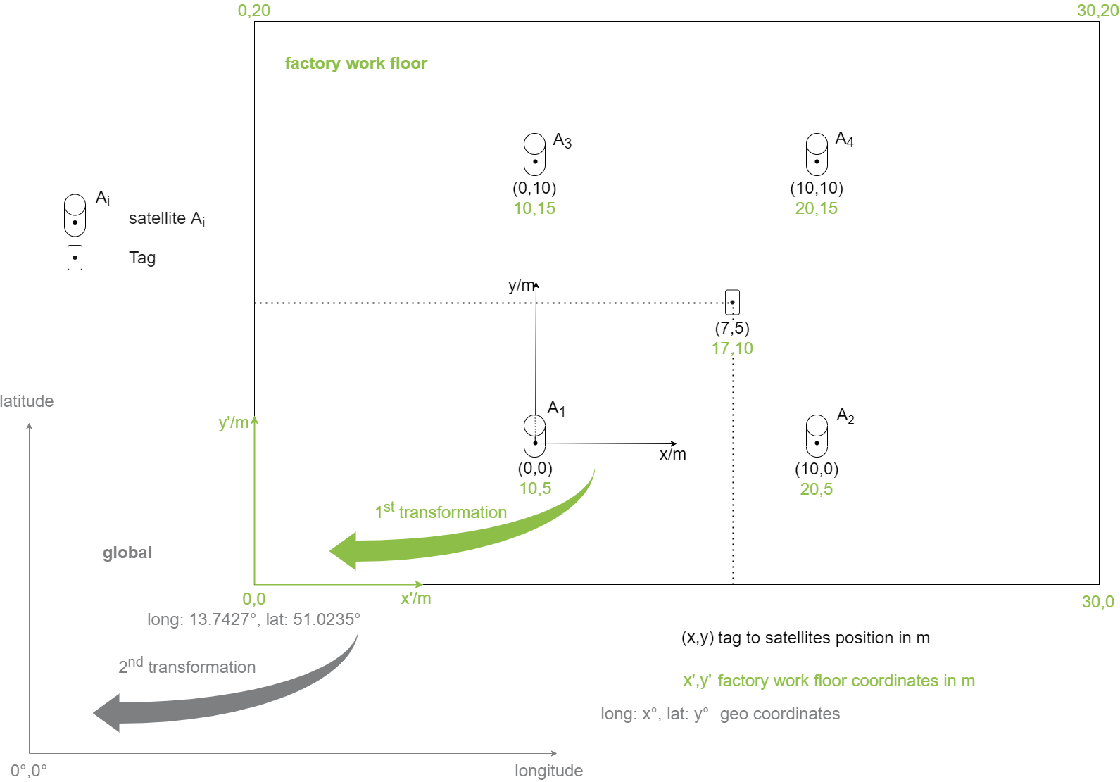
In this first part, however, we restrict ourselves to position determination in the plane, since the principles of the methods can be explained and illustrated more comprehensibly. In general, localization can be considered as a two- or multi-step procedure, where in the first step a relative position indication is determined from ranging values based on time stamps or time differences. This relative position information has a spatial reference to a hierarchically superordinate reference system or to absolute reference positions, so that in the second or further steps a transformation into the superordinate reference system up to absolute geo-coordinates can take place and we obtain an absolute position on the earth’s surface.
Example factory hall: First, the position of a tool within the factory hall is determined via a selected ranging procedure. This can be done e.g. via several distance measurements of the tool to fixed reference positions, satellites Ai. The determined coordinates, e.g. x=17m, y=10m of the tool indicate the relative position of the tool within the workshop with coordinate origin in one of the corners. The coordinate origin of the hall itself has absolute geo-coordinates, so that an absolute position on the earth’s surface can be assigned to the work part via transformation.
In a narrower sense, the position of the mobile object, tag, to the satellites is already to be regarded as a relative position. Accordingly, the first transformation already takes place from the tag-to-satellite coordinate system to the hall coordinates. This step is usually sufficient for industrial positioning.
Structure of a UWB message
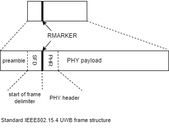
For the localization of objects in the UWB, several messages are exchanged between devices necessary for localization. These contain information crucial for localization. To send and receive one message in the UWB, two devices are needed, one acting as a transmitter, the other as a receiver. Usually, both devices are capable of transmitting and receiving messages. They are therefore referred to as transceivers. The basic structure of UWB messages is regulated by IEEE802.15.4 and looks as follows.
Time of Arrival (ToA)
The RMARKER in the sender and receiver message marks the end of the preamble and the beginning of the data package (payload). It is stored as a timestamp and can be transmitted in the payload. The time at which the RMARKER is detected at the receiving antenna is called Time of Arrival (ToA).
Signal propagation time - Time of Flight (ToF)
In order to determine distances between transmitters and receivers, the measurement of signal propagation time forms the basis in UWB-based RTL systems. The propagation time required by a signal from transmitter to receiver antenna is referred to as Time of Flight (ToF) and is determined by the difference in the timestamps at the transmitter and receiver antennas. The signals themselves travel through space as electromagnetic waves approximately at the speed of light c.
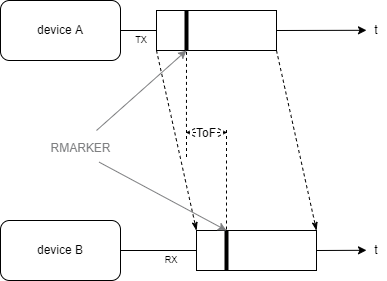
If the time of transmission and reception are known, the distance between transmitter and receiver can be determined via the signal propagation time (ToF):
$$ D = c \cdot \text{ToF} $$
If only one message is transmitted from device A to device B, as in the picture above, this is called One-Way-Ranging, which requires extremely precise time synchronization between transmitter and receiver. Extensions of this simple variant are explained below.
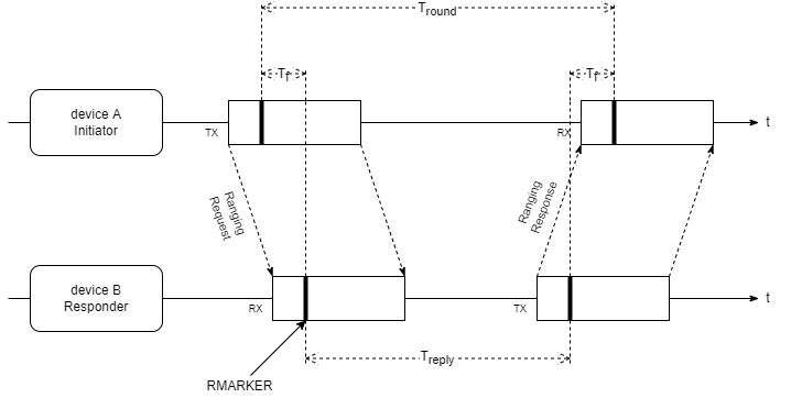
Single-Sided Two-Way-Ranging (SS-TWR)
In this method, the transmitter initiates the distance determination with a ranging request to the receiver, which receives it after the ToF (TF) and replies to the initiator with the response delay Treply. This so-called round trip is completed after the time Tround and the distance can be determined:
$$ D = \frac{c}{2} \cdot (T_\text{round}-T_\text{reply}) $$
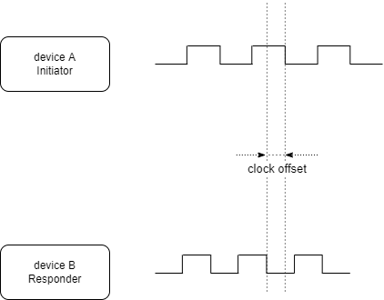
Since this is an asynchronous, asymmetrical method and the clocks on the transmitter and receiver side deviate from the nominal clock by up to 20ppm (worst case according to IEEE802.15.4a), the method leads to a clock offset between transmitter and receiver. It can therefore lead to enormous deviations of the determined distance to the true value.
An example: with a response delay of Treply=0.5ms and clock frequency of the UWB ICs of 125MHz we get for the deviation1 of the ToF from the true value: $$\hat T_\text{f} - T_\text{f} = \frac{T_\text{reply}}{2} (e_\text{A}-e_\text{B}) = \frac{0.5 \text{ ms}}{2} \cdot 40 \cdot 10^{-6} = 10 \text{ ns} $$ This corresponds to a distance deviation of 3 meters!
However, this problem can be gradually limited by certain procedures.
- detection:
- Hardware integrated clock offset ratio (COR) - detection of the received signal.
- via additional time measurement the time offset from transmitter to receiver can be determined
- correction:
- can be done on the software side by including the determined COR in the calculation of the distance
- can be done on hardware level by integrating a voltage controlled oscillator (VCO).
Examples:
- if the hardware integrated COR detection is used, this value can be read via a register of the UWB module. The calculation of the distance is done with correction of the clock offset: $$ D = \frac{c}{2} \cdot (T_\text{round}-(1-\text{COR}) \cdot T_\text{reply}) $$
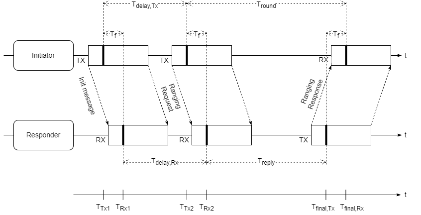
- If we send an additional message to the responder before the round trip, time differences on the sender and receiver side between the first and second message can be determined. In the second step, the COR can also be determined and the distance calculation corrected. The following time curve is intended to illustrate this:
By correcting the COR error, the time bases of the transmitter and receiver are aligned. The distance can be calculated as follows: $$ D = \frac{c}{2} \cdot (T_\text{round}-(1-\text{COR}) \cdot T_\text{reply})$$ $$= \frac{c}{2} \cdot \left(T_\text{final,Rx}-T_\text{Tx2} - \frac{T_\text{Tx2}-T_\text{Tx1}}{T_\text{Rx2}-T_\text{Rx1}} \cdot (T_\text{final,TX}-T_\text{Rx2})\right)$$
Double-Sided Two-Way-Ranging (DS-TWR)
The DS-TWR is an extension of the SS-TWR by an additional round trip, where device A first and device B in the second round trip take the role of the initiator.
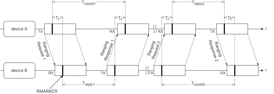
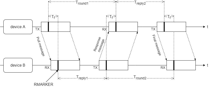
Four messages are transmitted between device A and B, which can be reduced to three, so that ranging is much faster and thus several measurements per time unit are possible. Thus Ranging Response 1, the end of the first round trip, can simultaneously make Ranging Request 2 and thus initiate the second round trip. In the DS-TWR with three messages, this message is called Ranging Response. Ranging is terminated with the final message, which contains all stored timestamps from device A in its message packet, to device B.
The distance can be determined for both variants with
$$ D=\frac{c}{4} \cdot (T_\text{round1}-T_\text{reply1}+T_\text{round2}-T_\text{reply2})$$
where the deviation from the true value of D is proportional to the clock offset (eA-eB) between the transmitter and receiver and the difference in the response delays (Treply2-Treply1). This means that the more the response delays of transmitter and receiver differ from each other, the larger the error is in our distance calculation.
Therefore the response delays need to be the same.
If this is the case, one speaks of symmetrical DS-TWR.
This requirement for symmetry is often difficult to realize. However, by a purely “mathematical trick” the distance between transmitter and receiver can also be given by
$$ D=c \cdot \left(\frac{T_\text{round1}T_\text{round2}-T_\text{reply1}T_\text{reply2}}{T_\text{round1}+T_\text{reply1}+T_\text{round2}+T_\text{reply2}}\right)$$
can be determined, where the strict requirement for symmetry does not apply. In this case, the response delays of both devices no longer have to be the same. This is referred to as asymmetric DS-TWR The distance error here is only proportional to the clock offset e and is therefore a maximum of 20ppm.
For further information, especially on formulas and their derivation, please refer to the following sources:
- D. Neirynck, E. Luk and M. McLaughlin, “An alternative double-sided two-way ranging method,” 2016 13th Workshop on Positioning, Navigation and Communications (WPNC), 2016, pp. 1-4, doi: 10.1109/WPNC.2016.7822844.
- “IEEE Standard for Wireless Medium Access Control (MAC) and Physical Layer (PHY) Specifications for Peer Aware Communications (PAC), Annex D” in IEEE Std 802.15.8-2017 , vol., no., pp.307-311, 7 Feb. 2018, doi: 10.1109/IEEESTD.2018.8287784.
Summary of ToF methods
The following table gives an overview of calculations with examples of the different TWR methods, their properties with advantages and disadvantages:
| $$ \hspace{2cm} $$ | SS-TWR | ||||
|---|---|---|---|---|---|
| symetric | asymmetric | ||||
| estimated ToF: $$ \hat T_\text{f} $$ | $$\frac{1}{2}(T_\text{round}-T_\text{reply})$$ | $$ \frac{1}{4} (T_\text{round1}-T_\text{reply1}+T_\text{round2}-T_\text{reply2})$$ | $$ \hspace{0.2cm} \frac{T_\text{round1}T_\text{round2}-T_\text{reply1}T_\text{reply2}}{T_\text{round1}+T_\text{reply1}+T_\text{round2}+T_\text{reply2}} $$ | ||
| with COR compensation: $$ \frac{1}{2}(T_\text{round}-(1-\text{COR})\cdot T_\text{reply}) $$ | |||||
| deviation1: $$\hat T_\text{f}-T_\text{f}$$ | $$\approx \frac{1}{2}(e_\text{A}-e_\text{B})T_\text{reply}$$ | $$\approx \frac{1}{4}(e_\text{A}-e_\text{B})(T_\text{reply2}-T_\text{reply1})$$ | $$e_\text{A}T_\text{f}=e_\text{B}T_\text{f}$$ | ||
| deviation: example | $$T_\text{reply}=0.5\text{ms}$$ deviation: 10ns \( \hat = \) 3m! | $$T_\text{reply2}-T_\text{reply1}=0.1\text{ms}$$ deviation: 1ns \( \hat =\) 30cm | $$ \hat T_\text{f}=300\text{ns} \; \hat = \; D=90\text{m}$$ deviation: 6ps \( \hat =\) 1.8mm | ||
| # messages | 2 or 3 with COR compensation | 3 or 4 | 3 or 4 | ||
| precision | – / + with COR compensation | + / ++ depending on symmetry | ++ | ||
| advantages | simple implementation | higher precision than SS-TWR | high precision, low requirement for synchrony | ||
| disadvantages | large deviation without COR compensation, strict requirements for synchrony | requirement for equal response delays complicates implementation | complexity in time and computing requirements | ||
Positioning with ToF
The position determination of a tag is based in the 2D case on a combination of at least one ToF measurement each between the tag and at least 3 satellites with their respective reference positions Ai. The determined distances Di between satellite and tag result in circles and map locations of equal signal propagation times (ToF). The intersection of the circles determines the position P of the tag.
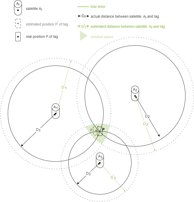
Due to measurement errors of the signal propagation times e.g. by the described clock offset, instead of an intersection point we get an intersection surface which allows a position estimation. The position determination in this solution space is done by mathematical methods, for ZIGPOS e.g. multi-dimensional scaling or probalistic by Monte-Carlo localization.
Time Difference of Arrival (TDoA)
This method is based on ToA in a narrower sense. The difference to the ToF method is that the reception times at the satellites are not used to determine signal propagation times (ToF) between transmitter and receiver, but time differences between the respective reception times at the receivers. One advantage of this is that the transmission time(s) do not have to be known and thus tags and satellites do not necessarily have to be clock synchronous. Satellites among each other, however, must be synchronized extremely precisely (in UWB time periods of 15.65ps).
Since it concerns time differences, we need, differently than with TWR, at least 3 transceivers, one tag and at least 2 satellites for a “distance determination”. Whereby the term “distance” is not correct here. Because a constant distance as with the ToF procedure to a certain satellite cannot be determined with the procedure. It is much more a matter of locations of equal signal propagation time differences and thus equal distance differences to two satellites. These locations can be determined as follows:
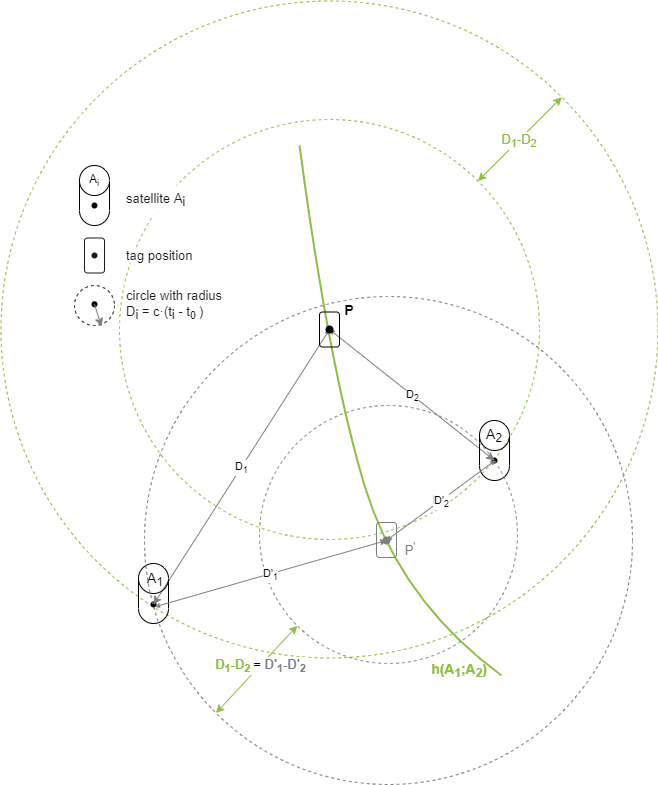
The tag transmits a signal at unknown time t0, which is detected at satellite Ai at time ti, and at satellite Aj at time tj. This results in circles with the radii Di and Dj; shown in the following figure. Although the individual radii on the hyperbola change, the difference between the radii is constant.
Once again: The drawn radii (distances from day to satellite) cannot be determined individually due to the unknown transmission time!
$$ h(A_\text{i};A_\text{j}): D_\text{i}-D_\text{j}=c \cdot (t_\text{i}-t_\text{0}) - c \cdot (t_\text{j}-t_\text{0}) = c \cdot (t_\text{i}-t_\text{j}) = \text{const.}$$
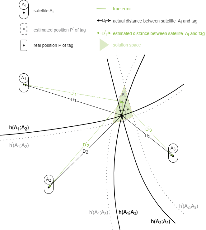
Positioning with TDoA
As with the ToF method, at least 3 satellites with their reference positions Ai are required in the 2D case to localize a tag. The hyperbolas h(Ai;Aj) denote the locations of equal time differences between satellite Ai and Aj as described before. For the localization of the tag, 2 hyperbolas are sufficient, since they give a unique intersection. However, 3 satellites result inevitably in 3 hyperbolas, so that all three are included in the position calculation. As with the ToA method, measurement errors h’(Ai;Aj) affect the estimation of tag position.
To understand how the hyperbolas evolve depending on the tag and satellite position, use the following interactive GeoGebra applet:
The applets used are based on the Anritsu TDOA simulation tool (Vers. 0.9) by Ferdinand Gerhardes.
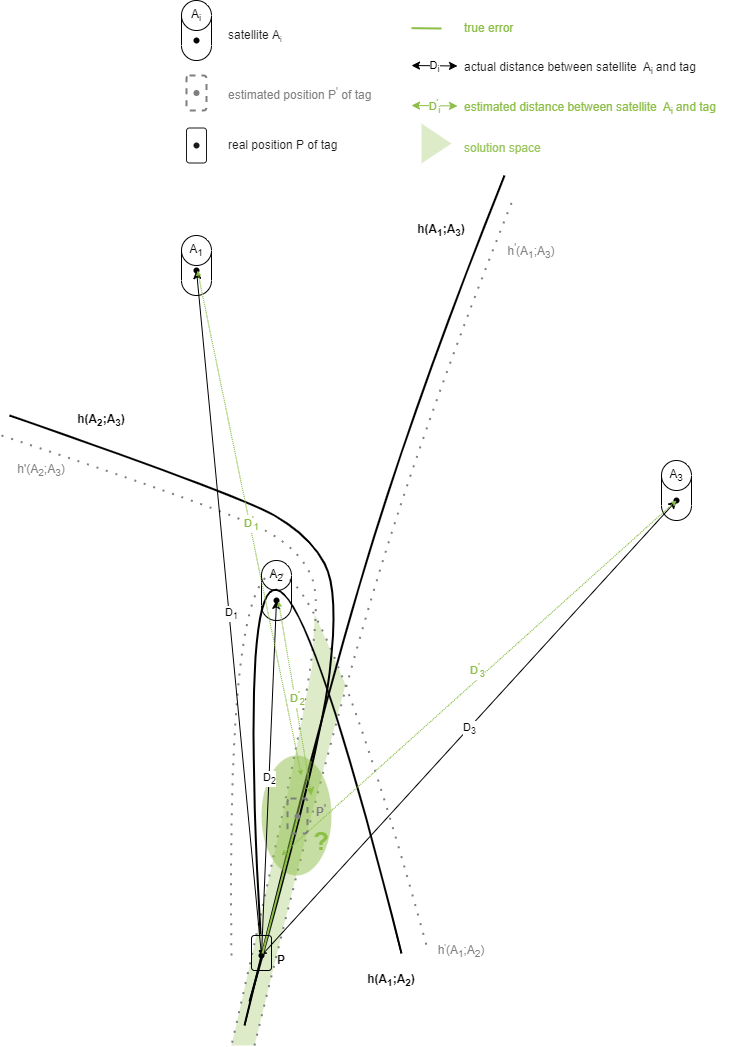
Robustness
Compared to the ToF-, the TDoA method is extremely susceptible to errors in the satellite boundary region. The error range or solution space for position estimation becomes larger and larger outside the satellite radii. The reason is the challenge in determining the hyperbolic intersection points. Since the solution space in ToF is determined using circles, the position estimation in the edge region is much more accurate than in TDoA. The following figure illustrates this.
Conclusion and summary
In this part, basic methods for distance determination between transmitters and receivers were described. These are based on signal propagation times or their differences. The localization takes place with the ToF over places of equal signal propagation times to the satellite (circles) and with the TDoA on places of equal signal propagation time differences between satellite pairs (hyperbolas). The methods for determining signal propagation times vary in complexity and their accuracies also differ depending on the topology.
We at ZIGPOS are constantly developing our RTLS in the interest of our customers. Besides precision, reliability and speed of our RTLS are always in the foreground for your satisfaction!
Read in the following part how we implement localization with the ZIGPOS RTLS.
-
The deviation is the difference between the estimated ToF derived from timestamps and the true ToF ( \( \hat T_\text{f} - T_\text{f} \) ) ↩︎